Showing posts with label Android. Show all posts

Saturday, June 20, 2015

Android BitTube

BitTube is a tiny AOSP (Android Open Source Project) class that I came upon while scouring the SensorService code.  It first piqued my interest because of its name, which I really like for some reason (do geeks really need reasons to like class names?).  But although the class is small, it felt like there was something interesting going on here, and that it will be worthwhile to do some digging.

If I came upon the BitTube class outside of the Android context, it would have been quite unremarkable and forgetful.  The BitTube implementation is pretty obvious and straight-forward: it is a "parcel-able" wrapper to a pair of sockets.  A socketpair to be exact.  And that's the eyebrow-raising tidbit: a socketpair is a Linux/Unix IPC (inter-process communication) mechanism very similar to a pipe.  What is a Linux IPC doing at the heart of AOSP when Binder is used almost everywhere else (another outlier is the RIL to rild - radio interface daemon - socket IPC)?

A socketpair sets up a two-way communication pipe with a socket attached to each end.  With file descriptor duplication (dup/dup2), you can pass the socket handle to another process, duplicate it and start communicating.  BitTube uses Unix sockets with sequenced packets (SOCK_SEQPACKET) which, like datagrams, only deliver whole records, and like SOCK_STREAM, are connection-oriented and guarantee in-order delivery.  Although socketpair  is a two-way communication pipe, BitTube uses it as a one-way pipe and assigns one end of the pipe to a writer and another to a reader (more on that later on).  The send and receive buffers are set to a default limit of 4KB each. There's an interface for writing and reading a sequence of same-size "objects" (sendObjects, recvObjects).

A short look around AOSP reveals that BitTube is used by the Display subsystem and by the Sensors subsystem, so let's look at how it is used the Sensors subsystem. I'll provide a very brief recap of the Sensors Java API to level-set, in case you are not familiar with this.
An application uses the SensorManager system service to access (virtual and physical) device sensors.   It registers to receive sensor events via two callbacks, which report an accuracy change or the availability of a sensor reading sample (event).

public class SensorActivity extends Activity, implements SensorEventListener {
     private final SensorManager mSensorManager;
     private final Sensor mAccelerometer;

     public SensorActivity() {
         mSensorManager = (SensorManager)getSystemService(SENSOR_SERVICE);
         mAccelerometer = mSensorManager.getDefaultSensor(Sensor.TYPE_ACCELEROMETER);
     }

     protected void onResume() {
         super.onResume();
         mSensorManager.registerListener(this, mAccelerometer, SensorManager.SENSOR_DELAY_NORMAL);
     }

     protected void onPause() {
         super.onPause();
         mSensorManager.unregisterListener(this);
     }

     public void onAccuracyChanged(Sensor sensor, int accuracy) {
     }

     public void onSensorChanged(SensorEvent event) {
     }
 }

There's a lot of work performed behind the scenes in order to implement the SensorManager.registerListener.  First, SensorManager delegates the request to SystemSensorManager which is the real workhorse.  I've copy-pasted the Lollipop code after removing some of the less-important, yet distracting code:

    /** @hide */
    @Override
    protected boolean registerListenerImpl(SensorEventListener listener, Sensor sensor,
            int delayUs, Handler handler, int maxBatchReportLatencyUs, int reservedFlags) {

        // Invariants to preserve:
        // - one Looper per SensorEventListener
        // - one Looper per SensorEventQueue
        // We map SensorEventListener to a SensorEventQueue, which holds the looper
        synchronized (mSensorListeners) {
            SensorEventQueue queue = mSensorListeners.get(listener);
            if (queue == null) {
                Looper looper = (handler != null) ? handler.getLooper() : mMainLooper;
                queue = new SensorEventQueue(listener, looper, this);
                if (!queue.addSensor(sensor, delayUs, maxBatchReportLatencyUs, reservedFlags)) {
                    queue.dispose();
                    return false;
                }
                mSensorListeners.put(listener, queue);
                return true;
            } else {
                return queue.addSensor(sensor, delayUs, maxBatchReportLatencyUs, reservedFlags);
            }
        }
    }

As you can see, a SensorEventQueue and Looper are created per registered SensorEventListener.
The SensorEventQueue is the object which eventually delivers sensor events to the application. This class diagram can give you some high-level grasp of the Java and native class hierarchy.


Because this blog entry is about BitTube and not about the Sensor subsystem, I'll jump over many details: eventually a native SensorEventQueue  is created.
The native SensorEventQueue uses a SensorEventConnection to bridge the process address-space gap and communicate with the native SensorService.  The BnSensorEventConnection (this is the server-side of the IPC) creates a BitTube and with it a socketpair. One of the socket handles is dup'ed ('dup' system call) by the BpSensorEventConnection and, voila: we have a communication pipe between the two processes, as depicted below.


As I mentioned above, the BitTube is used as a one-way pipe: events are written on one side and read by the SensorEventQueue, on the other side.

During the construction of the socketpair 2 x 4KB (default size) buffers are allocated by the kernel (one for the send-side buffer and the other for the receive-side buffer) using the SO_SNDBUF and SO_RCVBUF socket options. Remember that this is done per SensorEventListener.  And there's also a Looper thread per SensorEventListener.  Quite a lot of overhead.
So, the question still begs, what's gained by using this "new" IPC?  At first I thought that this was some legacy design from the early days of Android, or perhaps from some module that was integrated some time ago into the code-base.  But this wouldn't explain why BitTube is also used by DisplayEventReceiver for what looks like a similar setup.
Maybe it provides extra low latency?  BitTube can deliver several events in one write/read, but that can also be done with Binder without introducing any complications.  They both incur about the same number of context switches, buffer copies, and system calls.
Is simplicity the motivation?  No, BitTube is about as complex as using Binder.
This leaves me with throughput as the only other reason I can think of.  But sensors are defined as low bandwidth components:

Not included in the list of physical devices providing data are camera, fingerprint sensor, microphone, and touch screen. These devices have their own reporting mechanism; the separation is arbitrary, but in general, Android sensors provide lower bandwidth data. For example, “100hz x 3 channels” for an accelerometer versus “25hz x 8 MP x 3 channels” for a camera or “44kHz x 1 channel” for a microphone.

For me, the mystery remains.  If you have some thoughts on this, please comment - I'd love to learn.
In any case, BitTube provides another tool in our AOSP tool chest - although I'm hesitant about using it, until I understand what extra powers it give me :-)

Saturday, April 18, 2015

Android's Graphics Buffer Management System (Part II: BufferQueue)

In the first post on Android's graphics buffer management, I discussed gralloc, which is Android's graphics buffer allocation HAL.  In this post I'll describe graphics buffers flows in Android, with special attention to class BufferQueue which plays a central role in graphics buffer management.

Introduction

Before I dive in, I want to discuss buffers in general.  There is a surprising number of details and aspects involved in designing buffer systems and I think it is best to examine what was done in Android once we've assumed a wide and generic perspective.
Data buffers, and specifically image and graphics data buffers, exist as part of a specific subsystem, such as the camera subsystem, but can also span multiple subsystems, such as buffers shared between the camera and video subsystems.  Buffers provide a means to temporarily store data to allow us to separate the production of data from the consumption of data - in both time and space. That is, we can produce (or collect) data at one moment, and use it at a different moment.  This decouples producer and consumer, and also allows producer and consumer to be asynchronous to one another.  Many times in an event-based system the data producer and the data consumer are triggered (clocked) by different time sources.  For example, the camera on your mobile phone produces image frames at some arbitrary frame-rate (e.g. 30 frames per second, of FPS) while the display panel (showing the preview) can operate at a different refresh-rate (e.g. 60 Hz).  Moreover, even if the devices were guaranteed to operate at the same frequency (or if one frequency is a harmonic of the other), they are unlikely to have the same phase offset since the display operation starts when we turn on the screen, while the camera operation starts at some other arbitrary time when we start the camera application. And of course there is drift and jitter that contribute the asynchronous nature of the two subsystems. There may also be several consumers, or several producers.  SurfaceFlinger, for example, uses buffers from multiple sources and composes them into a single output buffer.

Buffers also allow us to move data from one part of our system to another.  Inevitably, buffers follow some paths within our system and these are commonly referred to the as the "data paths".  A path can start at a buffer provider which allocates new memory or provides a buffer from a pre-allocated pool. The buffers are considered empty at this stage.  That is, they do not contain consumable data or metadata. A source entity provides the initial data by attaching it to a buffer (reference holding buffers) or copying the data to the buffer's memory.  Somehow, a buffer makes its way along a path of buffer handlers until it arrives at the content consumer which uses the data and discards the buffer. A buffer handler may be passive (e.g. monitor or logger), or it be active: filtering (drop), altering, augmenting, extracting, or otherwise manipulating the contents.  These paths can be either dynamic or static.  There are many design patterns which define how a data path is defined and controlled (pipes and filters, layering, pipeline, software bus messaging, direct addressing, broadcasting, observing, and so forth) and I will not cover them here as that would really be diverging from our topic.

Buffer systems are either closed-looped or open-looped.  In closed-loop paths there is a buffer path from the consumer back to the producer.  Sometimes this is made explicit, and sometimes implicit. For example, if the producer and consumer use a shared memory pool they implicitly form a closed-loop.    One can argue that using a shared buffer pool is not really a closed-loop, but I contend that as long as the system is designed using explicit knowledge of shared buffer memory, then it is closed. That is, if the consumer can starve or delay the producer because it controls the flow of buffers available to the producer, then this is a closed-loop system. C

Ah, and there is the question of what we mean by buffer.  A lot of time when people say "buffer" they are referring to the actual backend memory storing the content, but in real systems it is quite rare to see raw data moving around the system.  It is much more common to see buffer objects which contain metadata describing the data content.  What is contained in this metadata is implementation-specific and depends on the problem domain and context, but I'm sure we can agree that one piece of information we need to know is the amount of data stored in the buffer.  And there is the question of pointer-to-data (by reference) vs embedded data (by value).  Obviously zero-copy buffer handling is preferred, but requires us to be exact about buffer memory life-time management.  Life time management, access management and synchronization are other related aspects which I've discussed in the previous post so I'll cut things short right here. 

BufferQueue

After this generic discussion of data buffers, we can finally dive into the Android details. I'll start with class BufferQueue because it is at the center graphic buffer movement in Android.  It abstracts a queue of graphics buffers, uses gralloc to allocate buffers, and has means to connect buffer producers and consumers which reside in different process address spaces.
Code for class BufferQueue and many of the cooperating classes that I'll be discussing can be found in directory /frameworks/native/libs/gui/ with the header files in /frameworks/native/include/gui.


Class BufferQueue has a static factory method, BufferQueue::createBufferQueue, which is used to create BufferQueue instances.

    // BufferQueue manages a pool of gralloc memory slots to be used by
    // producers and consumers. allocator is used to allocate all the
    // needed gralloc buffers.
    static void createBufferQueue(sp* outProducer,
            sp* outConsumer,
            const sp& allocator = NULL);

A quick glance at the implementation reveals that class BufferQueue is only a thin facade to class BufferQueueCore, which conatins the actual implementation logic.  For simplicity of this discussion, I will not make a distinction between these classes.

Working with BufferQueue is pretty straight-forward.  First, producers and consumers connect to the BufferQueue.
1. The producer takes an “empty” buffer from the BufferQueue (dequeueBuffer)
2. The producer (e.g. camera) copies image or graphics data into the buffer
3. The producer returns the “filled” buffer to the BufferQueue (queueBuffer)
4. The consumer receives an indication (via callback) of the presence of a “filled” buffer
5. The consumer removes this buffer from the BufferQueue (acquireBuffer)
6. When the consumer is done consuming the buffer is returned to the BufferQueue (releaseBuffer)

The following diagram shows a simplified interaction diagram between the camera (image buffer producer) and the display (image buffer consumer). 

Figure 1: Simplified data path between the camera subsystem and the GPU
Producers and Consumers may reside in different processes and this is accomplished using Binder, as always.

BufferQueueProducer is the workhorse behind IGraphicBufferProducer.  BufferQueueProducer maintains an intimate relationship with BufferQueueCore and directly accesses its member variables, including mutexes, conditions and other significant members (such as its pointer to IGraphicBufferAlloc).  Personally, I don't like this - it is confusing and fragile. 
When a Producer is requested to provide an empty buffer using dequeueBuffer, it tries to fetch one from BufferQueueCore which maintains an array of buffers and their states (DEQUEUED, QUEUED, ACQUIRED, FREE).  If a free slot is found in the buffer array but it doesn’t contain a buffer, or if the Producer was explicitly asked to reallocate the buffer, then BufferQueueProducer uses BufferQueueCore’s to allocate a new buffer.  

Initially, all invocations of dequeueBuffer results in the allocation of new buffers.  But because this is a closed-loop system, where the buffer Consumer returns buffers once it has consumed their contents (by calling releaseBuffer), we should see the system reaching equilibrium after a very short while.  Be aware that although BufferQueueCore can maintain an array of variable-sized GraphicBuffer objects, it is wise to make all buffers of the same size.  Otherwise, each invocation of dequeueBuffer may require the allocation of a new GraphicBuffer instance.

Figure 2: The main classes related to BufferQueue
 The GraphicBuffer allocation is performed using an implementation of IGraphicBufferAlloc which is provided to BufferQueueCore when it is constructed.  The default implementation of IGraphicBufferAlloc is provided by SurfaceFlinger (the system object in charge of composing all surfaces) and uses gralloc to allocate buffers.  In the previous post I discussed why a central graphics buffers allocator is well-advised when dealing with various hardware SoC modules.
Class BufferQueueCore doesn’t directly store GraphicBuffer – it uses class BufferItem which contains a pointer to a GraphicBuffer instance, including various other metadata (see frameworks/native/include/gui/BufferItem.h).
Figure 3: Class diagram showing the main classes related to graphics buffer allocation

Asynchronous notification interfaces IConsumerListener and IProducerListener are used to alert listeners about events such as a buffer being ready for consumption (IConsumerListener::onFrameAvailable); or the availability of an empty buffer (IProducerListener::onBufferReleased).  These callback interfaces also use Binder and can cross process boundaries.  Checkout further details in frameworks/native/include/gui/IConsumerListener.h

The best source of information I found on Android’s graphics system, aside from the code itself of course, is here.

Consumers

Figure: Some consumer classes

BufferQueue Creation

Figure: Top to bottom BufferQueue creation flow


Saturday, March 21, 2015

Android's Graphics Buffer Management System (Part I: gralloc)

In this post series I'll do a deep dive into Android's graphics buffer management system.  I'll cover how buffers produced by the camera use the generic BufferQueue abstraction to flow to different parts of the system, how buffers are shared between different hardware modules, and how they traverse process boundaries.
But I will start at buffer allocation, and before I describe what triggers buffer allocation and when, let's look at the low-level graphics buffer allocator, a.k.a. gralloc.

gralloc: Buffer Allocation

The gralloc is part of the HAL (Hardware Abstraction Layer) which means that the implementation is platform-specific.  You can find the interface definitions in hardware/libhardware/include/hardware/gralloc.h.  As expected from a HAL component, the interface is divided into a module interface (gralloc_module_t) and a  device interface (alloc_device_t).  Loading the gralloc module is performed as for all HAL modules, so I won't go into these details because they can be easily googled.  But I will mention that the entry point into a newly loaded HAL module is via the open method of the structure hw_module_methods which is referenced by the structure hw_module_t.  Structure hw_module_t acts as a mandatory "base class" (not quite since this is "C" code) of all HAL modules including gralloc_module_t.
Both the module and the device interfaces are versioned.  The current module version is 0.3 and the device version is 0.1.  Only Google knows why these interfaces have these sub-1.0 interface versions. :-)

As I said above, gralloc implementations are platform-specific and for reference you can look at the goldfish device's implementation (device/generic/goldfish/opengl/system/gralloc/gralloc.c).  Goldfish is the code name for the Android emulation platform device.
The sole responsibility of the device (alloc_device_t) is allocation (and consequent release) of buffer memory so it has a straight-forward  signature:

typedef struct alloc_device_t {
    struct hw_device_t common;

    /*
     * (*alloc)() Allocates a buffer in graphic memory with the requested
     * parameters and returns a buffer_handle_t and the stride in pixels to
     * allow the implementation to satisfy hardware constraints on the width
     * of a pixmap (eg: it may have to be multiple of 8 pixels).
     * The CALLER TAKES OWNERSHIP of the buffer_handle_t.
     *
     * If format is HAL_PIXEL_FORMAT_YCbCr_420_888, the returned stride must be
     * 0, since the actual strides are available from the android_ycbcr
     * structure.
     *
     * Returns 0 on success or -errno on error.
     */

    int (*alloc)(struct alloc_device_t* dev,
            int w, int h, int format, int usage,
            buffer_handle_t* handle, int* stride);
    /*
     * (*free)() Frees a previously allocated buffer.
     * Behavior is undefined if the buffer is still mapped in any process,
     * but shall not result in termination of the program or security breaches
     * (allowing a process to get access to another process' buffers).
     * THIS FUNCTION TAKES OWNERSHIP of the buffer_handle_t which becomes
     * invalid after the call.
     *
     * Returns 0 on success or -errno on error.
     */

    int (*free)(struct alloc_device_t* dev,
            buffer_handle_t handle);

    /* This hook is OPTIONAL.
     *
     * If non NULL it will be caused by SurfaceFlinger on dumpsys
     */
    void (*dump)(struct alloc_device_t *dev, char *buff, int buff_len);
    void* reserved_proc[7];
} alloc_device_t;

Lets examine the parameters for the alloc() function.  The first parameter (dev) is of course the instance handle.

The next two parameters (w, h) provide the requested width and height of the buffer.  When describing the dimensions of a graphics buffer there are two points to watch for.  First, we need to understand the units of the dimensions.  If the dimensions are expressed in pixels, as is the case for gralloc, then we need to understand how to translate pixels to bits.  And for this we need to know the color encoding format.

The requested color format is the forth parameter.  The color formats that Android supports are defined in /system/core/include/system/graphics.h.  Color format HAL_PIXEL_FORMAT_RGBA_8888 uses 32 bits for each pixel (8 pixels for each of the pixel components: red, green, blue and alpha-blending), while HAL_PIXEL_FORMAT_RGB_565 uses 16 bits for each pixel (5 bits for red and blue, and 6 bits for green).

The second important factor affecting the physical dimensions of the graphics buffer is its stride. Stride is the last parameter to alloc and it is also an out parameter.  To understand stride (a.k.a. pitch), it is easiest to refer to a diagram:


We can think of memory buffers as matrices arranged in rows and columns of pixels.  A row is usually referred to as a line.  Stride is defined as the number of pixels (or bytes, depending on your units!) that need to be counted from the beginning of one buffer line, to the next buffer line.  As the diagram above shows, the stride is necessarily at least equal to the width of the buffer, but can very well be larger than the width.  The difference between the stride and the width (stride-width) is just wasted memory and one takeaway from this is that the memory used to store an image or graphics may not be continuous.  So where does the stride come from?  Due to hardware implementation complexity, memory bandwidth optimizations, and other constraints, the hardware accessing the graphics memory may require the buffer to be a multiple of some number of bytes.  For example, if for a particular hardware module the line addresses need to align to 64 bytes, then memory widths need to be multiples of 64 bytes.  If this constraint results in longer lines than requested, then the buffer stride is different from the width. Another motivation for stride is buffer reuse: imagine that you want to refer to a cropped image within another image.  In this case, the cropped (internal) image has a stride different than the width.


Allocated buffer memory can be written to, or read from, by user-space code of course, but first and foremost it is written to, or read from, by different hardware modules such as the GPU (graphics processing unit), camera, composition engine, DMA engine, display controller, etc.  On a typical SoC these hardware modules come from different vendors and have different constraints on the buffer memory which all need to be reconciled if they are to share buffers.  For example, a buffer written by the GPU should be readable by the display controller.  The different constraints on the buffers are not necessarily the result of heterogeneous component vendors, but also because of different optimization points.  In any case, gralloc needs to ensure that the image format and memory layout is agreeable to both image producer and consumer.  This is where the usage parameter comes into play.

The usage flags are defined in file gralloc.h.  The first four least significant bits (bits 0-3) describe how the software reads the buffer (never, rarely, often); and the next four bits (bits 4-7) describe how the software writes the buffer (never, rarely, often).  The next twelve bits describe how the hardware uses the buffer: as an OpenGL ES texture or OpenGL ES render target; by the 2D hardware blitter, HWComposer, framebuffer device, or HW video encoder; written or read by the HW camera pipeline; used as part of zero-shutter-lag camera queue; used as a RenderScript Allocation; displayed full-screen on an external display; or used as a cursor.
Obviously there may be some coupling between the color format and the usage flag.  For example, if the usage parameter indicates that the buffer is written by the camera and read by the video encoder, then the format must be agreeable by both HW modules.
If software needs to access the buffer contents, either for read or write, then gralloc needs to make sure that there is a mapping from the physical address space to the CPU's virtual address space and that the cache is kept coherent.
For a sample implementation, you can examine the goldfish device implementation at /device/generic/goldfish/opengl/system/gralloc/gralloc.cpp.

Other factors affecting buffer memory

There are other factors affecting how graphic and image memory is allocated and how images are stored (memory layout) and accessed which we should briefly review:
Alignment
Once again, different hardware may impose hard or soft memory alignment requirements.  Not complying with a hard requirement will result in the failure of the hardware to perform its function, while not complying with a soft requirement will result in an sub-optimal use of the hardware (usually expressed in power, thermal and performance).

Color Space, Formats and Memory Layout
There are several color spaces of which the most familiar ones are YCbCr (images) and RGB (graphics).  Within each color space information may be encoded differently.  Some sample RGB encodings include RGB565 (16 bits; 5 bits for red and blue and 6 bits for green), RGB888 (24 bits) or ARGB8888 (32 bits; with the alpha blending channel).  YCbCr encoding formats usually employ chroma subsampling.
Because our eyes are less sensitive to color than to gray levels, the chroma channels can have a lower sampling rate compared to the luma channel with little loss of perceptual quality.  The subsampling scheme used does not necessarily dictate the memory layout.  For example, for 4:2:0 subsampling formats NV12 and YV12 there are two very different memory layouts, as depicted in the diagram below.

YV12 color - format memory layout (planar)
NV12 color - format memory layout (packed)
There are two YUV formats: packed formats (also known as semi-planar) and planar formats. NV12 is an example of a packed format, and YV12 is an example of a planar format.  In a packed format, the Y, U, and V components are stored in a single array. Pixels are organized into groups of macropixels, whose layout depends on the format. In a planar format, the Y, U, and V components are stored as three separate planes.
In the YV12 diagram above the Y (luma) plane has size equal to width * height, and each of the chroma planes (U, V) has a size equal to width/2 * height/2.  This means that both width and height must be even integers.  YV12 also stipulates hat the line stride must be a multiple of 16 pixels. Because both NV12 and YV12 are 4:2:0 subsampled, for each 2x2 group of pixels, there are 4*Y samples and 1*U and 1*V samples.

Tiling 
If the SoC hardware uses algorithms which mostly access blocks of neighboring pixels, then it is probably more efficient to arrange the image's memory layout such that neighboring pixels are laid out in line, instead of their usual position.This is called tiling.
Some graphics/imaging hardware use more elaborate tiling, such as supporting two tile sizes: a group of small tiles might be arranged in some scan order inside a larger tile.

Tiling: one the left is the image with the pixels in their natural order.  The green frame defines the 4x4 tile size and the red arrow shows the scan order.  On the right is the same image, but now with pixels arranged in the tile scan order.

Compression
If both producer and consumer are hardware components on the same SoC, then the may write and read a common, proprietary compressed data format and decompress the data on-the-fly (i.e. using on-chip memory, usually SRAM, just before processing the pixel data).

Memory Contiguity
Some older imaging hardware modules (cameras, display, etc) don't have an MMU or don't support scatter-gather DMA.  In this case the device DMA is programmed using physical addresses which point to contiguous memory.  This does not affect the memory layout, but it is certainly the kind of platform-specific constraint that gralloc needs to be aware of when it allocates memory.

gralloc: Buffer Ownership Management

Memory is a shared resource.  It is either shared between the graphics hardware module and the CPU; or between two graphics modules.  If the CPU is rendering to a graphics buffer, we have to make sure that the display controller waits for the CPU to complete writing, before it begins reading the buffer memory.  This is done using system-level synchronization which I'll discuss in a later blog entry.  But this synchronization is not sufficient to ensure that the display controller will be accessing a coherent view of the memory.  In the above example, the final updates to the buffer that the CPU writes may not have been flushed from the cache to the system memory.  If this happens, the display might show an incorrect view of the graphics buffer.  Therefore, we need some kind of low-level atomic synchronization mechanism to explicitly manage the transfer of memory buffer ownership which verifies that the memory "owner" sees a consistent view of the memory.

Access to buffer memory (both read and write, for both hardware and software)  is explicitly managed by gralloc users (this can be done synchronously or asynchronously).  This is done by locking and unlocking a buffer memory patch.  There can be many threads with a read-lock concurrently, but only one thread can hold a write lock.

    /*
     * The (*lock)() method is called before a buffer is accessed for the
     * specified usage. This call may block, for instance if the h/w needs
     * to finish rendering or if CPU caches need to be synchronized.
     *
     * The caller promises to modify only pixels in the area specified
     * by (l,t,w,h).
     *
     * The content of the buffer outside of the specified area is NOT modified
     * by this call.
     *
     * If usage specifies GRALLOC_USAGE_SW_*, vaddr is filled with the address
     * of the buffer in virtual memory.
     *
     * Note calling (*lock)() on HAL_PIXEL_FORMAT_YCbCr_*_888 buffers will fail
     * and return -EINVAL.  These buffers must be locked with (*lock_ycbcr)()
     * instead.
     *
     * THREADING CONSIDERATIONS:
     *
     * It is legal for several different threads to lock a buffer from
     * read access, none of the threads are blocked.
     *
     * However, locking a buffer simultaneously for write or read/write is
     * undefined, but:
     * - shall not result in termination of the process
     * - shall not block the caller
     * It is acceptable to return an error or to leave the buffer's content
     * into an indeterminate state.
     *
     * If the buffer was created with a usage mask incompatible with the
     * requested usage flags here, -EINVAL is returned.
     *
     */
 
    int (*lock)(struct gralloc_module_t const* module,
            buffer_handle_t handle, int usage,
            int l, int t, int w, int h,
            void** vaddr);
/*
     * The (*lockAsync)() method is like the (*lock)() method except
     * that the buffer's sync fence object is passed into the lock
     * call instead of requiring the caller to wait for completion.
     *
     * The gralloc implementation takes ownership of the fenceFd and
     * is responsible for closing it when no longer needed.
     */
    int (*lockAsync)(struct gralloc_module_t const* module,
            buffer_handle_t handle, int usage,
            int l, int t, int w, int h,
            void** vaddr, int fenceFd);


Cache Coherence
If software needs to access a graphics buffer, then the correct data needs to be accessible to the CPU for reading and/or writing.  Keeping the cache coherent is one of the responsibilities of gralloc. Needlessly flushing the cache, or enabling bus snooping on some SoCs, to keep the memory view consistent across graphics hardware and CPU wastes power and can add latency.  Therefore, here too, gralloc needs to employ platform-specific mechanisms.

Locking Pages in RAM
Another aspect of sharing memory between CPU and graphics hardware is making sure that memory pages are not flushed to the swap file when they are used by the hardware.  I can't remember seeing Android on a device configured with a swap file, but it is certainly feasible, and lock() should literally lock the memory pages in RAM.
A related issue is page remapping which happens when a virtual page that is assigned to one physical page, is dynamically reassigned a different physical page (page migration).  One reason the kernel might choose to do this is to prevent fragmentation by rearranging the physical memory allocation. From the CPU's point of view this is fine as long as the new physical page contains the correct content.  But from the point of a graphics hardware module, this is pulling the rug under its feet. Pages shared with hardware should be designated non-movable.


Friday, September 5, 2014

Google's Depth Map (Part II)

In the previous post I described Google's Lens Blur feature and how we can use code to extract the depth map stored in the PNG image output by Lens Blur.  Lens Blur performs a series of image frame captures, calculates the depth of each pixel (based on a user-configurable focus locus) and produces a new image having a bokeh effect.  In other words, the scene background, is blurred.  Lens Blur stores the new (bokeh) image, the original image, and the depth-map in a single PNG file.  

In this blog post we'll pick up where we left off last time, right after we extracted the original image and the depth map from the Lens Blur's PNG output file and stored them each in a separate PNG file.  This time we'll go in the reverse direction: that is, starting with the original image and the depth map we'll create a depth blurred image - an image with the bokeh effect.  I'm going to show that with very little sophistication we can achieve some pretty good results in replicating the output of Lens Blur.  This is all going to be kinda crude, but I think the RoI (return-on-investment) is quite satisfactory.

The original image as extracted to a PNG file
My simpleton's approach for depth blurring is this: I start by finding the mean value of the depth map.  As you probably recall, the grey values in the depth map correspond to the depth values calculated by Lens Blur.  The mean depth value will serve as a threshold value - every pixel above the threshold will be blurred while all other pixels will be left untouched.  This sounds rather crude, not to say dirty, but it works surprisingly well.  At the outset I thought I would need to use several threshold values, each with a differently sized blurring kernel.  Larger blurring kernels use more neighboring pixels and therefore increase the blurring effect.  But alas, a simple Boolean threshold filter works good enough.

The depth map as calculated by Lens Blur after extraction and storage as a PNG file.
The grey value of every pixel in this image corresponds to the depth of the pixel in
the original image.  Darker pixels are closer to the camera and have a smaller value.
The diagram below shows the Boolean threshold filter in action: we traverse all pixels in the original image an every pixel above the threshold is zeroed (black).

The result of thresholding the original image using the mean value of the depth-map.
You can see that the results are not too shabby.  Cool, right?

I think it is interesting to ask if it is legitimate to expect this thresholding technique to work for every Lens Blur depth-map? And what's the optimal threshold, I mean why not threshold using the median? or mean-C? or some other calculated value?
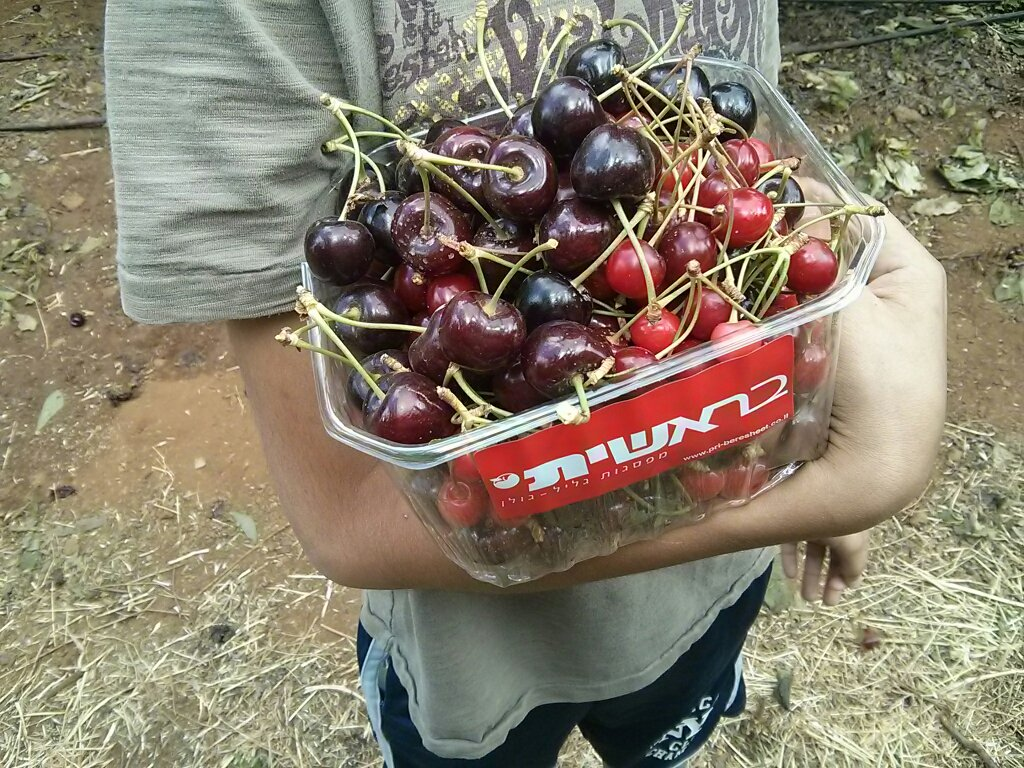
Let's get back to the image above: along the edges of the t-shirt and arm there is (as expected) a sharp gradient in the depth value.  Of course, this is due to Google's depth extraction algorithm which performs a non-gradual separation between foreground and background.  If we looked at the depth-map as a 3D terrain map, we should see a large and fast rising "mountain" where the foreground objects are (arm, cherry box).  We expect this "raised" group of pixels to be a closed and connected convex pixel set.  That is, we don't expect multiple "mountains" or sprinkles of "tall" pixels.  Another way to look at the depth-map is through the histogram.  Unlike intensity histograms , which tell the story of the image illumination, the data in our histogram conveys depth information.

The x-axis of the histogram depicted here (produced by IrfanView) is a value between 0-255 and corresponds to the height value assigned by Lens Blur (after normalizing to the 8-bit sample size space).  The y-axis indicates the number of pixels in the image which have the corresponding x values.  The red line is the threshold; here I located it at x=172 which is the mean value in the depth-map.  All pixels above the threshold (i.e. to the right of the red line) are background pixels and all pixels below the threshold are foreground.  This histogram looks like a classic bimodal histogram with two modes of distribution; one corresponding to the foreground pixels and the other corresponding to the background pixels.  Under the assumptions I laid above on how the Lens Blur depth algorithm works, this bimodal histogram is what we should expect.
It is now clear how the thresholding technique separates these two groups of pixels and how the choice of threshold value affects the results.  Obviously the threshold value needs to be somewhere between the foreground and the background modes.  Exactly where?  Now that's a bit tougher.  In his book on image processing, Alan Bovik suggests applying probability theory to determine the optimal threshold (see pages 73-74). Under our assumption of only two modes (background and foreground), and if we assume binomial probability density functions for the two modes, then Bovik's method is likely to work.  But I think the gain is small for the purpose of this proof-of-concept.  If you download the source code you can play around with different values for the threshold.

The next step is not much more complicated.  Instead of zeroing (blackening) pixels above the threshold, we use some kind of blurring (smoothing) algorithm, as in image denoising.  The general idea is to use each input pixel's neighboring pixels in order to calculate the value of the corresponding output pixel.  That is, we use convolution to apply a low-pass filter on the pixels which pass the threshold test condition.

Application of a filter on the input image to generate the output image.

As you can see in the code, I've used several different smooothing kernels (mean, median, gausian) with several different sizes.  There are a few details that are worth mentioning.
The convolution filter uses pixels from the surrounding environment of the input pixel, and sometimes we don't have such pixels available.  Let's take for example the first pixel, at the upper left corner (x,y) = (0,0) and a box kernel of size 5x5.  Clearly we are missing the 2 upper rows (y=-1, y=-2) and 2 left columns (x=-1, x=-2).  There are several strategies to deal with this such duplicating rows and columns or using a fixed value to replace the missing data.  Another strategy is to create an output image that is smaller than the input image.  For example, using the 5x5 kernel, we would ignore the first and last two rows and first and last two columns and produce an output image that is 4 columns and 4 rows smaller than the input frame.  You can also change the filter kernel such that instead of using the center of the kernel as the pixel we convolve around, we can use one of the corners.  This doesn't bring us out of the woods, but it lets us "preserve" two of the sides of the image.  And you can do what I did in the code, which is literally "cutting some corners": for all pixels in rows and columns that fall outside of a full kernel, I simply leave them untouched.  You can really see this when using larger kernels - the frame is sharp and the internal part of the image is blurry.  Ouch - I wouldn't use that in "real" life ;-)
Next, there's the issue of the kernel size.  As mentioned above, larger kernel sizes achieve more blurring, but the transition between blurred pixels and non-blurred pixels (along the depth threshold contour lines) is more noticeable.  One possible solution is to use a reasonably sized kernel and perform the smoothing pass more than once.  If your filter is non-linear (e.g. Gaussian) then the result might be a bit hairy.
In the output of Google's Lens Blur you can also easily detect artifacts along the depth threshold contour lines, but because they change the "strength" of the blurring as a function of the pixel depth (instead of a binary threshold condition as in my implementation) they can achieve a smoother transition at the edges of the foreground object.

Gaussian smoothing with kernel size 9x9

Mean.filter with 7x7 kernel size., 2 passes
Mean.filter with 11x11 kernel size., 1 pass
Mean.filter with 15x15 kernel size., 1 pass

Overall, this was quite a simple little experiment, although the quality of the output image is not as good as Lens Blur's.  I guess you do get what you pay for ;-)


/*
 *  The implementation is naive and non-optimized to make this code easier to read
 *  To use this code you need to download LodePNG(lodepng.h and lodepng.cpp) from 
 *  http://lodev.org/lodepng/.
 *  Thanks goes to Lode Vandevenne for a great PNG utility!
 *
 */
#include "stdafx.h"
#include "lodepng.h"
#include 
#include 
#include 
#include 
#include 

struct image_t {
    image_t() : width(0), height(0), channels(0), buf(0) {}
    image_t(size_t w, size_t h, size_t c, uint8_t *buf ) : 
        width(w), height(h), channels(c), buf(buf) {}
    size_t width;
    size_t height;
    size_t channels;
    uint8_t *buf;
};

struct box_t {
    box_t(size_t w, size_t h) : w(w), h(h) {}
    size_t w;
    size_t h;
};

struct image_stats {
    image_stats() : mean(0) {
        memset(histogram, 0, sizeof(histogram));
    }
    size_t histogram[256];
    size_t mean;
};

void calc_stats(image_t img, image_stats &stats) {
    uint64_t sum = 0;  // 64 bit sum to prevent overflow

    // assume the image is grayscale and calc the stats for only the first channel
    for (size_t row=0; row v;
        for (size_t y=row-size.h/2; y<=row+size.h/2; y++) {
            for (size_t x=col-size.w/2; x<=col+size.w/2; x++) {
                v.push_back( 
                   input.buf[y*input.width*input.channels + x*input.channels + color]);
            }
        }
        std::nth_element( v.begin(), v.begin()+(v.size()/2),v.end() );
        return v[v.size()/2];
    }
};


class Gaussian_9x9 : public Filter {
public:
    Gaussian_9x9(const image_t &input, const image_t &output) : 
        Filter(input, output, box_t(9,9)) {}
private:
    size_t convolve(size_t row, size_t col, size_t color) const {
        static const 
        uint8_t kernel[9][9] = {{0, 0, 1,  1,  1,  1, 1, 0, 0}, 
                                {0, 1, 2,  3,  3,  3, 2, 1, 0}, 
                                {1, 2, 3,  6,  7,  6, 3, 2, 1}, 
                                {1, 3, 6,  9, 11,  9, 6, 3, 1}, 
                                {1, 3, 7, 11, 12, 11, 7, 3, 1}, 
                                {1, 3, 6,  9, 11,  9, 6, 3, 1}, 
                                {1, 2, 3,  6,  7,  6, 3, 2, 1}, 
                                {0, 1, 2,  3,  3,  3, 2, 1, 0}, 
                                {0, 0, 1,  1,  1,  1, 1, 0, 0}};
        static const size_t kernel_sum = 256;
        size_t total = 0;
        for (size_t y=row-size.h/2; y<=row+size.h/2; y++) {
            for (size_t x=col-size.w/2; x<=col+size.w/2; x++) {
                total += input.buf[y*input.width*input.channels + x*input.channels + 
                                   color] * 
                         kernel[y-row+size.h/2][x-col+size.w/2];
            }
        }
         return total/kernel_sum;
    }
};

class Gaussian_5x5 : public Filter {
public:
    Gaussian_5x5(const image_t &input, const image_t &output) : 
        Filter(input, output, box_t(5,5)) {}
protected:
    size_t convolve(size_t row, size_t col, size_t color) const {
        static const 
        uint8_t kernel[5][5] = {{ 1,  4,  7,  4,  1},
                                { 4, 16, 26, 16,  4},
                                { 7, 26, 41, 26,  7},
                                { 4, 16, 26, 16,  4},
                                { 1,  4,  7,  4,  1}};
        static const size_t kernel_sum = 273;
        size_t total = 0;
        for (size_t y=row-size.h/2; y<=row+size.h/2; y++) {
            for (size_t x=col-size.w/2; x<=col+size.w/2; x++) {
                // convolve
                total += input.buf[y*input.width*input.channels + x*input.channels + 
                                   color] * 
                          kernel[y-row+size.h/2][x-col+size.w/2];
            }
        }
        return total/kernel_sum;
    }
};

void blur_image(const image_t &input_img, const image_t &output_img, 
                const image_t &depth_img, const BlurConfig &cfg) {
  size_t width = input_img.width;
  size_t height = input_img.height;
  size_t channels = input_img.channels;

  for (size_t pass=cfg.num_passes; pass>0; pass--) {
      for (size_t row=0; row cfg.threshold) {
                    size_t new_pixel = cfg.filter.execute(row, col, color);    
                    output_img.buf[row*width*channels+col*channels+color] = new_pixel;
                } else {
                    output_img.buf[row*width*channels + col*channels + color] = 
                        input_img.buf[row*width*channels + col*channels + color];
                }
            }
        }
      }
      // going for another pass: the input for the next pass will be the output 
      // of this pass
      if ( pass > 1 ) 
        memcpy(input_img.buf, output_img.buf, height*width*channels);
  }
 }

void do_blur() {
    const std::string wdir("");
    const std::string inimage(wdir + "gimage_image.png");
    const std::string outimage(wdir + "gimage_image.blur.png");
    const std::string depthfile(wdir + "gimage_depth.png");

    image_t depth_img;
    depth_img.channels = 3;
    unsigned error = lodepng_decode24_file(&depth_img.buf, &depth_img.width, 
                                           &depth_img.height, depthfile.c_str());
    if(error) { 
        printf("[%s] decoder error %u: %s\n", depthfile.c_str(), error, 
                lodepng_error_text(error));
        return;
    }

    image_t input_img;
    input_img.channels = 3;
    error = lodepng_decode24_file(&input_img.buf, &input_img.width, 
                                  &input_img.height, inimage.c_str());
    if(error) { 
        printf("[%s] decoder error %u: %s\n", depthfile.c_str(), error, 
                lodepng_error_text(error));
        return;
    }

    image_t output_img(input_img.width, 
                       input_img.height, 
                       input_img.channels, 
                       (uint8_t *) 
                       malloc(input_img.width*input_img.height*input_img.channels));
    
    image_stats depth_stats;
    calc_stats(depth_img, depth_stats);
    // Choose one of these filters or add your own
    // Set the filter connfiguration: filter algo and size, number of passes, threshold
    BlurConfig cfg(MeanBlur(input_img, output_img, box_t(7,7)), 3, depth_stats.mean);
    /*
    BlurConfig cfg(MeanBlur(input_img, output_img, box_t(11,11)), 2, depth_stats.mean);
    BlurConfig cfg(MedianBlur(input_img, output_img, box_t(7,7)), 1, depth_stats.mean);
    BlurConfig cfg(Constant(input_img, output_img), 1, depth_stats.mean);
    BlurConfig cfg(Gaussian_9x9(input_img, output_img), 1, depth_stats.mean);
    BlurConfig cfg(Gaussian_5x5(input_img, output_img), 5, depth_stats.mean);
    */

    blur_image(input_img, output_img, depth_img, cfg);

    error = lodepng_encode24_file(outimage.c_str(), output_img.buf, 
                                  output_img.width, output_img.height);
    if (error) 
        printf("[%s] encoder error %u: %s\n", outimage.c_str(), error, 
                lodepng_error_text(error));

    free(depth_img.buf);
    free(input_img.buf);
    free(output_img.buf);
}

int main(int argc, char* argv[])
{
    do_blur();
    return 0;
}

Saturday, June 7, 2014

Google's Depth Map


In my previous post I reported on Android's (presumed) new camera Java API and I briefly mentioned that its purpose is to provide the application developer more control over the camera, therefore allowing innovation in the camera application space. Google's recent updates to the stock Android camera application includes a feature called Lens Blur, which I suspect uses the new camera API to capture the series of frames required for the depth-map calculation (I am pretty sure that Lens Blur is only available on Nexus phones, BTW). In this post I want to examine the image files generated by Lens Blur.

Google uses XMP extended JPEG for storing Lens Blur picture files. The beauty of XMP is that arbitrary metadata can be added to a file without causing any problems for existing image viewing applications. Google's XMP's based depth-map storage format is described by Google on their developer pages but not all metadata fields are actually used by Lens Blur; and not all metadata used by Lens Blur are described on the developer pages. To look closer at this depth XMP format, you can copy a Len Blur image (JPEG) from your Android phone to your PC and open the file using a text editor. You should see the XMP metadata similar to the pasted data below:

<x:xmpmeta xmlns:x="adobe:ns:meta/" x:xmptk="Adobe XMP Core 5.1.0-jc003">
  <rdf:RDF xmlns:rdf="http://www.w3.org/1999/02/22-rdf-syntax-ns#">
    <rdf:Description rdf:about=""
        xmlns:GFocus="http://ns.google.com/photos/1.0/focus/"
        xmlns:GImage="http://ns.google.com/photos/1.0/image/"
        xmlns:GDepth="http://ns.google.com/photos/1.0/depthmap/"
        xmlns:xmpNote="http://ns.adobe.com/xmp/note/"
      GFocus:BlurAtInfinity="0.0083850715"
      GFocus:FocalDistance="18.49026"
      GFocus:FocalPointX="0.5078125"
      GFocus:FocalPointY="0.30208334"
      GImage:Mime="image/jpeg"
      GDepth:Format="RangeInverse"
      GDepth:Near="11.851094245910645"
      GDepth:Far="51.39698028564453"
      GDepth:Mime="image/png"
      xmpNote:HasExtendedXMP="7CAF4BA13EEBAC578997926C2A696679"/>
  </rdf:RDF>
</x:xmpmeta>


<x:xmpmeta xmlns:x="adobe:ns:meta/" x:xmptk="Adobe XMP Core 5.1.0-jc003">
  <rdf:RDF xmlns:rdf="http://www.w3.org/1999/02/22-rdf-syntax-ns#">
    <rdf:Description rdf:about=""
        xmlns:GImage="http://ns.google.com/photos/1.0/image/"
        xmlns:GDepth="http://ns.google.com/photos/1.0/depthmap/"
        GImage:Data="/9j/4AAQSkZJRQABAAD/2wBDAAUDBAQEAwUEBAQFBQUGBwwIBw...."
         GDepth:Data="iVBORw0KGgoAAAANSUhEUgAABAAAAAMACAYAAAC6uh......"
  </rdf:RDF>
</x:xmpmeta>

Two fields, GImage:Data and GDepth:Data are particularly interesting. The former stores the original image which I suppose is one of the series of images captured by the application. The latter stores the depth map as described by Google and as annotated by the metadata in the first RDF structure. The binary JPEG data that follows is the image that is actually displayed by the viewer and it is not necessarily the same picture that is stored in GImage:Data because this may be the product of a Lens Blur transformation. Storing the original picture data, with the depth-map and the "blurred" image takes a lot of room, but gives you the freedom to continuously alter the same picture. It is quite a nice feature.

Figure 1: Lens Blur output
Figure 2: image data stored in GImage:Data.
Notice that the background is very sharp compared to figure 1.

Figure 3: Depth map as extracted from GDepth:Data
GImage:Data and GDepth:Data are XML text fields so they must be encoded textually somehow, and Google chose to use Base64 for the encoding. When I decoded these fields I found that the image data (GImage:Data) stores a JPEG image, and the depth-map (GDepth:Data) is stored in a PNG image.

The following code extracts GImage:Data and GDepth:Data into two separate files (having JPEG and PNG formats, respectively). It starts by opening the Lens Blur file and searching for either GDepth:Data= or GImage:Data=. It then proceeds to decode the Base 64 data and spits out the decoded data into new files. It is quite straight forward except for a small caveat: interspersed within the GDepth:Data and GImage:Data is some junk that Google inserted in the form of a name-space URL descriptor (http://ns.adobe.com/xmp/extension/), a hash value, and some binary valued-bytes. I remove these simply by skipping 79 bytes once I detect a 0xFF byte.

// Naive O(n) string matcher
// It is naive because it always moves the "cursor" forward - even when a match fails.
// This is a correct assumption that we can make in the context of this program.
bool match(std::ifstream &image, const std::string &to_match) {
    size_t matched = 0;
    while (!image.eof()) {
        char c;
        image.get(c);
        if (image.bad())
            return false;
        if (c == to_match[matched]) {
            matched++;
            if (matched==to_match.size())
                return true;
        }
        else {
            matched = 0;
        }
    }
    return false;
}

class Base64Decoder {
public:
    Base64Decoder() : base64_idx(0) {}
    bool add(char c);
    size_t decode(char binary[3]);
private:
    static int32_t decode(char c);
    char base64[4];
    size_t base64_idx;
};


bool Base64Decoder::add(char c) {
    int32_t val = decode(c);
    if (val < 0)
        return false;

    base64[base64_idx % 4] = c;
    base64_idx = ++base64_idx % 4;
    if (base64_idx % 4 == 0) {
        return true;
    }
    return false;
}

inline
size_t Base64Decoder::decode(char binary[3]) {
    if (base64[3] == '=')  {
        if (base64[3] == '=') {
            int32_t tmp = decode(base64[0]) << 18;
                         
            binary[2] = binary[1] = 0;
            binary[0] = (tmp>>16) & 0xff;
            return 1;
        } else {
            int32_t tmp = decode(base64[0]) << 18 |
                          decode(base64[1]) << 12;
                         
            binary[2] = 0;
            binary[1] = (tmp>>8) & 0xff;
            binary[0] = (tmp>>16) & 0xff;
            return 2;
        }
    }

    int32_t tmp = decode(base64[0]) << 18 |
                  decode(base64[1]) << 12 |
                  decode(base64[2]) << 6  |
                  decode(base64[3]);

    binary[2] = (tmp & 0xff);
    binary[1] = (tmp>>8) & 0xff;
    binary[0] = (tmp>>16) & 0xff;
    return 3;
}


// Decoding can be alternatively performed by a lookup table
inline
int32_t Base64Decoder::decode(char c) {
    if (c>= 'A' && c<='Z')
        return (c-'A');
    if (c>='a' && c<='z')
        return (26+c-'a');
    if (c>='0' && c<='9')
        return (52+c-'0');
    if (c=='+')
        return 62;
    if (c=='/')
        return 63;
     
    return -1;
}

bool decode_and_save(char *buf, size_t buflen, Base64Decoder &decoder, std::ofstream &depth_map) {
    size_t i = 0;
    while (i < buflen) {
         // end of depth data
        if (buf[i] == '\"')
            return true;

        if (buf[i] == (char)0xff) {
            // this is Google junk which we need to skip
            i += 79; // this is the length of the junk
            assert(i        }

        if (decoder.add(buf[i])) {
            char binary[3];
            size_t bin_len = decoder.decode(binary);
            depth_map.write(binary, bin_len);
        }
        i++;
    }
    return false;
}

void extract_depth_map(const std::string &infile, const std::string &outfile, bool extract_depth) {
    std::ifstream blur_image;
    blur_image.open (infile, std::ios::binary | std::ios::in);
    if (!blur_image.is_open()) {
        std::cout << "oops - file " << infile << " did not open" << std::endl;
        return;
    }

    bool b = false;
    if (extract_depth)
        b = match(blur_image, "GDepth:Data=\"");
    else
        b = match(blur_image, "GImage:Data=\"");
    if (!b) {
        std::cout << "oops - file " << infile << " does not contain depth/image info" << std::endl;
        return;
    }

    std::ofstream depth_map;
    depth_map.open (outfile, std::ios::binary | std::ios::out);
    if (!depth_map.is_open()) {
        std::cout << "oops - file " << outfile << " did not open" << std::endl;
        return;
    }
   
    // Consume the data, decode from base64, and write out to file.
    char buf[10 * 1024];
    bool done = false;
    Base64Decoder decoder;
    while (!blur_image.eof() && !done) {
        blur_image.read(buf, sizeof(buf));
        done = decode_and_save(buf, sizeof(buf), decoder, depth_map);
    }

    blur_image.close();
    depth_map.close();
}

void main() {
    const std::string wdir(""); // put here the path to your files
    const std::string infile(wdir + "gimage_original.jpg");
    const std::string imagefile(wdir + "gimage_image.jpg");
    const std::string depthfile(wdir + "gimage_depth.png");

   extract_depth_map(infile, depthfile, true);
   extract_depth_map(infile, imagefile, false);
}

If you want to use the depth-map and image data algorithmically (e.g. to generate your own blurred image), don't forget to decompress the JPEG and PNG files, otherwise you will be accessing compressed pixel data. I used InfranView to generate raw RBG files, which I then manipulated and converted back to BMP files. I didn't include this code because it is not particularly interesting. Some other time I might describe how to use Halide ("a language for image processing and computational photography") to process the depth-map to create new images.